Understanding Histograms, Mean & Standard Deviation in Drone Mapping & 3D Point Cloud Analysis

Statistics are the mathematical backbone of wildlife conservation and ecology. They allow researchers to estimate population sizes, track migration patterns, understand animal behaviour, and evaluate the impacts of environmental changes or human activity on ecosystems. Here is how key statistical concepts are used in the field, followed by an explanation of the mean and standard deviation.

How Statistics are used in Wildlife

• Population Estimation: Instead of counting every single animal (which is usually impossible), biologist’s use statistical sampling and capture-mark-recapture models to accurately estimate total population sizes.
• Habitat Modelling: Researchers use statistical regression to analyse environmental variables (like temperature, vegetation, and water proximity) to predict where specific species are most likely to live or roam.
• Conservation Monitoring: Statistical tests help determine if a population is growing, shrinking, or staying stable over time, and whether conservation efforts (like anti-poaching patrols) are actually working.

1. Mean

The mean, commonly known as the average, is the central value of a data set.

• How it works: You find the mean by adding all the numbers in your data set together and dividing by the total count of those numbers.
• Wildlife example: If you record the number of eggs laid in 5 different sea turtle nests, let’s say nest 1 = 105 eggs, nest 2 = 110 eggs, nest 3 = 98 eggs, nest 4 = 115 eggs and nest 5 = 102 eggs. We add the number of egg and divide by the number of nests: (105+110+98+115+102)/5 = 106 eggs. The Mean or average number of eggs is 106.

2. Standard Deviation

The standard deviation measures the amount of variation or “spread” in a set of data.

• Low standard deviation: The data points are clustered closely around the mean (most numbers are very similar).
• High standard deviation: The data points are spread out over a wide range of values (the numbers are very different from one another).

Wildlife example: The sample standard deviation for this data is 6.67 eggs (rounded to two decimal places).

In wildlife biology, we use the sample standard deviation because we are looking at a small subset (5 nests) instead of every sea turtle nest on Earth.

Step-by-Step Calculation

Here is exactly how that number is calculated:

1. Find the mean: The mean is 106 eggs, as calculated before.
2. Subtract the mean from each number of eggs in the nest to find the deviation for each nest:
   • 105 – 106 = -1
   • 110 – 106 = 4
   • 98 – 106 = -8
   • 115 – 106 = 9
   • 102 – 106 = -4
3. Square each of those deviations (to remove negative numbers):
   • (-1)² = 1
   • (4) ² = 16
   • (-8) ² = 64
   • (9) ² = 8
   • (-4) ² = 16
4. Sum the squared values: 1 + 16 + 64 + 81 + 16 = 178
5. Divide by n – 1 where n is the number of samples, so 5 – 1 = 4:
   • 178/4 = 44.5*
6. Take the square root of that result (return the number to its original unit of measurement after square of deviations which removed negatives):
   • √44.5 = ±6.67

*Why n -1 and not just n?

Our Standard deviation (spread) either side (±) of the mean (average) is 6.67 eggs. We subtract 1 from the number of samples—a correction known as Bessel’s Correction—to account for the fact that a small sample usually underestimates the true variation of the entire population.

Here is exactly why this mathematical adjustment is necessary.

1. Samples Tend to Underestimate Variation

When you collect a small sample (like 5 turtle nests), the animals or nests you measure are highly likely to come from the main, average part of the population.

You are very unlikely to accidentally pick the absolute extremes—such as the single largest or single smallest turtle nest on the entire beach. Because your sample lacks these rare extremes, the raw spread of your data looks smaller than it actually is in the wild.

2. The Role of the Sample Mean

To calculate standard deviation, you must first calculate the sample mean (106 eggs).

Because that mean is generated from your 5 sample nests, the data points are mathematically closer to their own sample mean than they would be to the true, unknown mean of all millions of turtle nests on Earth.

If you divide by just n, you get a biased result that falsely suggests your data is more tightly clustered than it really is. Dividing by n-1 makes the denominator smaller, which mathematically inflates the standard deviation just enough to correct this bias.

3. Degrees of Freedom

In statistics, this concept is called degrees of freedom.

Imagine you have 5 data points, and you already know their mean is 106.

• The first 4 nests can have any number of eggs imaginable (they are free to vary).
• However, once those first 4 numbers are locked in, the 5th nest has to be a specific number to make the average come out to exactly 106.

Therefore, only n-1 (4 out of 5) of your data points are truly free to vary. The last data point holds no new informational value regarding variation.

Sample vs. Population

Biologists use two different formulas depending on what they are studying:

• Use n-1 (Sample): When you look at a subset of a group (e.g., 5 nests to estimate the whole beach). This is almost always used in wildlife biology.
• Use n (Population): Only when you have counted literally every single individual in existence (e.g., if there are only 5 Kakapo parrots left in a specific sanctuary and you measured all 5).

3. Histograms

A histogram is a graph that shows how frequently different values occur in a dataset.

The x-axis represents the measured values, while the y-axis shows how many observations fall within each range of values.

Histograms are powerful because they reveal the shape of a dataset. While the mean tells us the average and the standard deviation tells us the spread, a histogram shows whether the data are evenly distributed or influenced by a small number of unusually large or small values.

The Significance of Statistics & drone data for vegetation recovery monitoring

Now let’s have a look at what this means with regards to drone data. A site was cleared of sensitive fynbos vegetation for construction. After clearing, the site was scanned using a DJI Phantom 4 Pro V2 and the image data proceeded in WebODM into high resolution maps and 3D point clouds. Construction of the site was put on hold indefinitely and therefore the fynbos had time to recover. 15 months later the site was scanned again in the exact same manner and the data aligned with the first data set and processed in WebODM.

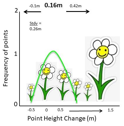
The two 3D point clouds were then analysed using Cloud Compares M3C2 tool to detect the change in vegetation over the site over the 15 month recovery period. The resulting stats showed a mean of 16cm and a standard deviation of 26cm. The standard deviation is larger than the mean itself, indicating substantial variation in vegetation growth across the site. But the resulting histogram shows us why. The overall recovery (vegetation growth) was generally small and uniform, but there were a few species that grew much taller, much faster over that time. This makes a lot of sense as there were a small number of invasive alien plants (Acacia mearnsii) as well as a small number of fast growing pioneer plants (Osteospermum moniliferum) that grew up to 1.5 metres over that time. Most of the site came up with smaller species such as Erica bicolour and the like.

Image 1: The histogram generated from the M3C2 change between data set 1 and 2. Count is the number of points in the point cloud and M3C2 distance is how many metres the points have changed between the two point clouds ove the 15 month period. Note the long tail to the right and the small increase in the number points measuring 1.3 to 1.5 metres. These likely represent the small number of fast-growing plants detected in the survey. There is a small number of points that shift towards the negative, this is most likely due to compaction and break down of sticks and rotting stumps.

Conclusion

A drone survey is far more than a collection of aerial photographs and attractive 3D models. When combined with statistical analysis and change detection tools such as M3C2, those datasets become powerful scientific records. They allow us to quantify ecological recovery, identify unusual patterns of growth, and monitor environmental change with a level of detail that would be difficult to achieve through traditional field methods alone. Understanding the statistics behind the data is what transforms a beautiful map into meaningful ecological insight.